Now since we’ve already worked through the chapter 4 book content in my lesson 3 blogpost, I won’t repeat the work here, instead I’d recommend you checkout that post if you’d like to see the book content that pairs with this week’s lecture.
Downloading Data from Kaggle
Building upon the concepts and principles we learned in lesson 3, we’re going to build our neural net from scratch and run it against the titanic dataset which we can source from kaggle. We can use the python api to select the competition and download all the data to a given path like we have below
Cool, we’ve got our test, train, and submission csvs as well as the original zip.
As mentioned in the lesson, we’re going to import pytorch and numpy to work with arrays, and pandas for working with dataframes
import torchimport numpy as npimport pandas as pd
Data Cleaning
Lets first do some data cleaning along with the course
df = pd.read_csv(path/"train.csv")
df.head()
PassengerId
Survived
Pclass
Name
Sex
Age
SibSp
Parch
Ticket
Fare
Cabin
Embarked
0
1
0
3
Braund, Mr. Owen Harris
male
22.0
1
0
A/5 21171
7.2500
NaN
S
1
2
1
1
Cumings, Mrs. John Bradley (Florence Briggs Thayer)
female
38.0
1
0
PC 17599
71.2833
C85
C
2
3
1
3
Heikkinen, Miss. Laina
female
26.0
0
0
STON/O2. 3101282
7.9250
NaN
S
3
4
1
1
Futrelle, Mrs. Jacques Heath (Lily May Peel)
female
35.0
1
0
113803
53.1000
C123
S
4
5
0
3
Allen, Mr. William Henry
male
35.0
0
0
373450
8.0500
NaN
S
As we learned in lesson 3, we want to apply all our inputs by some weights and biases, but if we look at the ‘Cabin’ column there are some ‘NaN’ values, or “Not a Number” values, we’ve got to change this to something computable for our model to work. Lets checkout how many NaNs are there in the whole dataset
df.isna().sum()
PassengerId      0
Survived         0
Pclass           0
Name             0
Sex              0
Age            177
SibSp            0
Parch            0
Ticket           0
Fare             0
Cabin          687
Embarked         2
dtype: int64
Ok it looks like only Age and Cabin have NaN values that we need to handle. One strategy for imputing missing values is replacing them with the ‘mode’, or the most commonly occuring value already present in the array, lets checkout the mode.
modes = df.mode().iloc[0]modes
PassengerId                      1
Survived                       0.0
Pclass                         3.0
Name           Abbing, Mr. Anthony
Sex                           male
Age                           24.0
SibSp                          0.0
Parch                          0.0
Ticket                        1601
Fare                          8.05
Cabin                      B96 B98
Embarked                         S
Name: 0, dtype: object
We can now fill the columns with the most commonly occuring values that we grabbed from above
df.fillna(modes, inplace=True)
Any empties left? Lets look
df.isna().sum()
PassengerId    0
Survived       0
Pclass         0
Name           0
Sex            0
Age            0
SibSp          0
Parch          0
Ticket         0
Fare           0
Cabin          0
Embarked       0
dtype: int64
The pandas describe() function is a really cool way to investigate either all or certain datatypes, combine this with numpy’s types and we can get specifically all the numeric data types by using the np.number base class and the describe() method
np.number?
Init signature: np.number()Docstring: Abstract base class of all numeric scalar types.
File: c:\users\nick\anaconda3\envs\fastai\lib\site-packages\numpy\__init__.py
Type: type
Subclasses: integer, inexact
df.describe(include=np.number)
PassengerId
Survived
Pclass
Age
SibSp
Parch
Fare
count
891.000000
891.000000
891.000000
891.000000
891.000000
891.000000
891.000000
mean
446.000000
0.383838
2.308642
28.566970
0.523008
0.381594
32.204208
std
257.353842
0.486592
0.836071
13.199572
1.102743
0.806057
49.693429
min
1.000000
0.000000
1.000000
0.420000
0.000000
0.000000
0.000000
25%
223.500000
0.000000
2.000000
22.000000
0.000000
0.000000
7.910400
50%
446.000000
0.000000
3.000000
24.000000
0.000000
0.000000
14.454200
75%
668.500000
1.000000
3.000000
35.000000
1.000000
0.000000
31.000000
max
891.000000
1.000000
3.000000
80.000000
8.000000
6.000000
512.329200
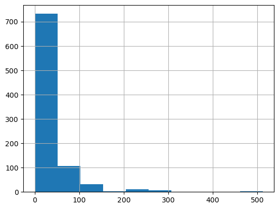
Ok we can see that fare has 75% of fares under \$31 but a mean of \$32 and a max of $512, this would lead us to thinking there’s quite a skewed distribution. This kind of skewness will bias our weights to these large values when we don’t really want them to, lets have a look at the distribution.
df.Fare.hist()
Super skewed! Almost all the values are below 50, yet we go up to ~\$500 in this graph. What we can do to distribute these values more normally is take the log of the array which will squish down these massive numbers and not fetter with the lower values too much. Also we’re adding 1 to all values since there are some 0 fares and log(0) is infinity.
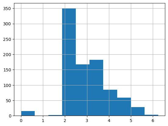
df["LogFare"] = np.log(df.Fare+1)
df.LogFare.hist()
That looks way better, sure its not perfect but everything is a more manageable value and we can definitely see a reduced skew.
Lets checkout the other columns
df.describe()
PassengerId
Survived
Pclass
Age
SibSp
Parch
Fare
LogFare
count
891.000000
891.000000
891.000000
891.000000
891.000000
891.000000
891.000000
891.000000
mean
446.000000
0.383838
2.308642
28.566970
0.523008
0.381594
32.204208
2.962246
std
257.353842
0.486592
0.836071
13.199572
1.102743
0.806057
49.693429
0.969048
min
1.000000
0.000000
1.000000
0.420000
0.000000
0.000000
0.000000
0.000000
25%
223.500000
0.000000
2.000000
22.000000
0.000000
0.000000
7.910400
2.187218
50%
446.000000
0.000000
3.000000
24.000000
0.000000
0.000000
14.454200
2.737881
75%
668.500000
1.000000
3.000000
35.000000
1.000000
0.000000
31.000000
3.465736
max
891.000000
1.000000
3.000000
80.000000
8.000000
6.000000
512.329200
6.240917
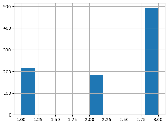
PClass also seems to only have three classes, which is actually outlined to us in the competition guidelines, we could also look at the histogram to see.
df.Pclass.hist()
Thats not continuous at all, we can also use the unique() method on the pandas dataframe
df.Pclass.unique()
array([3, 1, 2], dtype=int64)
pclasses =sorted(df.Pclass.unique())pclasses
[1, 2, 3]
Ok now lets checkout the non numeric values, which we’ll have to represent numerically somehow since we need to be able to multiply them by our weights and biases. A simple way to do this is one-hot-encoding them, also known as making ‘dummy’ values which creates a binary column each for ‘n’ classes and then a 0 or 1 in each column if that class is observed. You can technically do n-1 classes since if all the binary columns are 0 then you’ve technically observed the last column but most often you’ll explicitly express each column.
Cumings, Mrs. John Bradley (Florence Briggs Thayer)
38.0
1
0
PC 17599
71.2833
C85
4.280593
1
0
1
0
0
1
0
0
2
3
1
Heikkinen, Miss. Laina
26.0
0
0
STON/O2. 3101282
7.9250
B96 B98
2.188856
1
0
0
0
1
0
0
1
3
4
1
Futrelle, Mrs. Jacques Heath (Lily May Peel)
35.0
1
0
113803
53.1000
C123
3.990834
1
0
1
0
0
0
0
1
4
5
0
Allen, Mr. William Henry
35.0
0
0
373450
8.0500
B96 B98
2.202765
0
1
0
0
1
0
0
1
Ok we can see some new columns being added, with the structure of ‘originalColumn_classObservation’, for example ‘Sex_female’. Lets grab these added columns specifically.
Now we’ve got to make our ‘x’ (Independent / Predictors) and ‘y’ (Dependent / Target) tensors for us to train and predict with. We’re trying to predict if someone survived so “Survived” is our y value.
from torch import tensort_dep = tensor(df.Survived)
Our x values are all the continues values we can grab as well as the dummy values we made.
Ok so we’ve got our 891 observations of 12 columns / attributes / features to work with.
Building our Linear Model
We will first build a totally linear model without any non-linear activation functions like a ReLu (That we worked through in Lesson 3), to do this we’ll get a coefficient for each independent variable (column/feature) by picking a random value in the range of (-5,5).
Our first column age is simply a lot bigger than all our other columns and is dominating the output, we can normalise the values between 0 and 1 for all columns so that no particular nominal size of values for any column is bigger than another. We can use sigmoid or simply divide by the maximum of the column to do this normalisation.
vals, indices = t_independent.max(dim=0)vals, indices
Awesome, everything is looking far more balanced now.
The course makes a great note to highlight the vector by matrix calculations we’re running here. Note that ‘t_independent’ is a matrix and coefficients is a vector of values, even though we’re simply saying multiply each other, pytorch knows to broadcast the vector over the whole matrix for the calculations. Definitely checkout lesson 3 / chapter 4 of the book to learn more about this. I’ve also linked some decent broadcasting documentation there as well.
As with lesson 3, we need a way to optimise those coefficients/weights and we do that via calculating a loss and gradients which we then multiply by a learning rate to move our coefficients/weights to a more effective value. Lets do that now.
loss = torch.abs(preds-t_dep).mean()loss
tensor(0.5372)
We’ve taken the absolute error of our predictions minus the true value and then grabbed the mean(). We’re pretty close to random chance at .53 since there can only be a 0 or 1 value.
Lets wrap calculating the predictions and losses in some helper functions and keep moving.
Here we’re going to manually do gradient descent, or a single ‘epoch’ of training. Pytorch will automatically track our gradients for us with the ‘requires_grad_()’ attribute on our coefficients so we don’t have to manually set them but you can handle this manually if you wish (which we did in lesson 3).
Gradients for free! So cool, Pytorch will add the gradients anytime our coefficients are involved in a function and calculate them for us, it will simply add them to the .grad attribute. Lets calculate the loss again and see them double
loss = calculate_loss(coefficients,t_independent, t_dep)loss.backward()coefficients.grad
Perfect, lets now modify our coefficients and zero out our gradients so that they don’t keep blowing up/doubling as we keep calculating. Lets also introduce our learning rate that will decide by how much to step our weights against the gradients. We’re going to modify our coefficients by subtracting the gradients by the learning rate
Our loss went down to .4774 from .5372, its working! We’re heading in the right direction
Training the Linear Model
As we worked through in lesson 3, we need to setup a validation set in order to see how well we’re performing on data that we haven’t seen, but this is separate from our test set which we keep separate until the very end. We can use the fastai RandomSplitter and simply use a random split in this case.
from fastai.data.transforms import RandomSplittertrain_split, validation_split = RandomSplitter(seed=26)(df)
From .539 error all the way down to .301, consistent and deliberate progress, good stuff.
Now considering we have a coefficient for each column, we can look at the coefficients and infer some knowledge of how each feature impacted someone’s chances for survival
How cool is that, we can see each column and the literal impact of increasing or decreasing each value on the survival of the person observed in the dataset.
Lets move on to measuring accuracy since we’re currently using absolute error whereas the competition actually uses accuracy.
Lets make the assumption that any passenger over 0.5 is predicted to survive, any prediction over 0.5 where the individual survived is correct in this case
Lets checkout the average accuracy over the whole set
results.float().mean()
tensor(0.7809)
78% accuracy considering we have only have 12 coefficients and a linear function is kind of amazing. Lets define a nice accuracy helper function so we can re-calculate this anytime
We do however have the problem of both below 0 and above 1 predictions which make no sense since 0 and 1 are limits. There’s a magical function call sigmoid that provides a way to smooth all our predictions between 0 and 1, lets do it!
Using Sigmoid
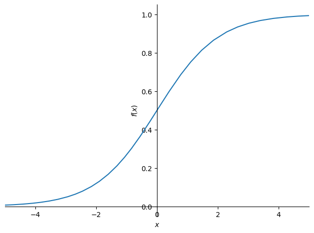
Sigmoid lets us nicely smooth everything between 0 and 1 whilst never actually reaching either, lets have a look at the function visually
We’re using this cool library called sympy which allows us to write an expression like we did above and have it nicely plotted. Similar to the plot_function() method from fastai but a whole library.
doc(sympy)
sympy
sympy
SymPy is a Python library for symbolic mathematics. It aims to become a
full-featured computer algebra system (CAS) while keeping the code as simple
as possible in order to be comprehensible and easily extensible. SymPy is
written entirely in Python. It depends on mpmath, and other external libraries
may be optionally for things like plotting support.
See the webpage for more information and documentation:
https://sympy.org
Pytorch already has sigmoid out the box so we don’t have to write up a custom method, it’ll do the awesome math on our GPU, all parallel and quick. Lets redefine our calculate_predictions method to include this.
We’ve been doing vector to matrix calculations, where we have to sum all the rows over axis ‘1’ to get our results, we can instead run a matrix multiplication on the vector by matrix and it will broadcast the vector over the entire matrix to achieve the same thing. We simply need to change our ’*’ operator to a ‘@’ operator
We produce the identical tensor and total but this is more efficient since we’re able to run these calculations in parallel on the GPU, lets modify our calculate_preds() again to reflect this
The only other thing we need to do is convert our vector to a matrix with a single column and ‘transpose’ it so that its a matrix by matrix calculation instead of a matrix by vector
Ok so we have our coefficients for each of our layers, we have a constant bias term, we can now make our neural network by handcrafting our layers and adding our non-linearities in between them before finally passing to sigmoid for our predictions.
import torch.nn.functional as Fdef calculate_preds(coefficients, independents): l1, l2, const = coefficients res = F.relu(independents@l1) res = res@l2 + constreturn torch.sigmoid(res)
Ok see here how we’re grabbing our layers, multiplying the independents by the first layer, multiplying that result by a relu activation (non-linearity is introduced here) and then finally multiplying by our final layer and adding our constant term. We then have our output which we can sigmoid to get our final prediction.
We also need to write our method to update the coefficients by calculating the gradients for each layer, subtracting them by the learning rate and zeroing out the gradients to be calculated in the next batch/epoch.
def update_coefficients(coefficients, learning_rate):for layer in coefficients: layer.sub_(layer.grad * learning_rate) layer.grad.zero_()
We’ve got everything together, lets quickly checkout our layers, remembering there’s a relu inbetween the layers and we have our final constant term
Layer one takes in our 12 ‘x’ values as the independent variables, outputs a shape of 20 which our next layer takes in and then condenses to 1 output which we sigmoid for our prediction. Hopefully these shapes make sense, and that bigger architectures are just more complicated connections between these matrices of different sizes and shapes which are suited better to particular problems.
Well our loss is definitely better at 0.195 but our accuracy is still the same which is interesting, whilst we haven’t blown away our linear model, its really cool to see how only a couple of layers of matrices can give effective results.
Making the Neural Net ‘Deep’
Now whilst the universal approximation paper says that two layers is all you need to approximate any function in the universe (a terrible paraphrase of what the paper says), its not very practical in the real world. It also isn’t very ‘deep’ since we only have two layers, by building more layers, we make our network ‘deep’, hence the name. Again we need to connect layer to layer with activations in between, lets do it.
Note that the sizes variables is our ‘crude’ model architecture, simply the structure of all the hidden layers (the model body) and the final output layer which spits out predictions is the (model head)
def initialise_coefficients(): hiddens=[12,5,12,5] sizes = [n_coefficients] + hiddens + [1] n =len(sizes) layers = [(torch.rand(sizes[i], sizes[i+1])-0.3)/sizes[i+1]*4for i inrange(n-1)] consts = [(torch.rand(1)[0]-0.5)*0.1for i inrange(n-1)]for l in layers+consts: l.requires_grad_()return layers, consts
As Jeremy notes in the course, there are lots of fiddly constants here, the initialisation of weights has drastic impacts on the training progress of your model, there are ways to address this which we’ll work on later through the course but its important to note these aren’t accidental and are part of the difficult nature of this type of model.
We’ll also re-define our calculate predictions method and loop through each layer instead of explicitly calling them
def calculate_preds(coefficients, independents): layers, consts = coefficients n =len(layers) res = independentsfor iteration, layer inenumerate(layers): res = res@layer + consts[iteration]if iteration!=n-1: res = F.relu(res)return torch.sigmoid(res)
Check it out, the line res = res@layer + consts[i] is our \(prediction = weights * inputs + bias\) or \(y = mx + b\) equation from lesson 3. Still blows my mind that these simple equations can be built up into such flexible models that are truly effective at solving problems.
We also need to update our coefficients updating method since we’ve got many layers and constants rather than explicit setups
Ok maybe this model architecture wasn’t as great as our two layers but its still cool to see how we can ‘artisinally’ create our layers and whats happening within each layer. This was a really interesting ‘double up’ on lesson 3 which covers the same chapter 4 of the book. I’m feeling very confident in the raw mechanices of how these models function which is fantastic. On to lesson 6 and thanks for reading if you’re here with me.