Lesson 4 | Natural Language Processing, Transformers, Huggingface

A New Library, New Model Architectures, And Natural Language Data

Checkout this notebook in colab

This week focuses on building models with interact with natural language which is very different from images or structured tabular data. Jeremy starts off discussing some model architectures (some of which he pioneered with collaborators) like ‘ULMFit’, ‘Transformers’, and Recurrent Neural Nets (RNNs) which are often seen in the news headlines as being significant. This week will also use huggingface, which is another library from fastai but is seemingly the best library as of writing this for working with language. We’re going to dive into tokenising and other natural language specific problems.

Lecture Content

US Patent Phrase Matching

We’re working with the US Patent Phrase Matching Kaggle Competition data for this lesson lecture, I’ve just visited the page and downloaded the dataset into my local data path but you can of course use the kaggle APIs.

This competition in particular is about comparing two short phrases and whether they are similar to each other based on which patent class they were used with. Scores of 1 being identical and 0 meaning they are different. The scores are represented in a set of 0, 0.25, 0.5, and 1 which acts like a classification problem rather than regression because they’re distinct instead of smooth.

Jeremy starts by proposing that we can feed this into our model successfully by representing the data as “TEXT1: abatement; TEXT2: eliminating process” of which we then pick a distinct category from the above. To my understand this relates to the ‘anchors’ and ‘target’ in this dataset which we’ll look at below.

EDA of Patent Data

from pathlib import Path
from fastai.vision.all import *

data_path = Path("../data/us-patent-phrase-to-matching/")

data_path.ls()

(#2) [Path('../data/us-patent-phrase-to-matching/test.csv'),Path('../data/us-patent-phrase-to-matching/train.csv')]

import pandas as pd

df = pd.read_csv(data_path / "train.csv")

df.head()

	id	anchor	target	context	score
0	37d61fd2272659b1	abatement	abatement of pollution	A47	0.50
1	7b9652b17b68b7a4	abatement	act of abating	A47	0.75
2	36d72442aefd8232	abatement	active catalyst	A47	0.25
3	5296b0c19e1ce60e	abatement	eliminating process	A47	0.50
4	54c1e3b9184cb5b6	abatement	forest region	A47	0.00

df.describe(include="object")

	id	anchor	target	context
count	36473	36473	36473	36473
unique	36473	733	29340	106
top	37d61fd2272659b1	component composite coating	composition	H01
freq	1	152	24	2186

From having a quick look at a data sample and a description of the dataframe itself, there simply aren’t that many unique contexts or anchors, and the anchor ‘component composite coating’ turns up 152 times which seems like a lot our of the 733 total.

Lets now build our first feature which will be the ‘input’ feature. We’ll structure this feature as we noted earlier in the TEXT1: …; TEXT2:…; format

df['input'] = "TEXT1: " + df.context + "; TEXT2: " + df.target + "; ANC1: " + df.anchor

df.input.head()

0    TEXT1: A47; TEXT2: abatement of pollution; ANC1: abatement
1            TEXT1: A47; TEXT2: act of abating; ANC1: abatement
2           TEXT1: A47; TEXT2: active catalyst; ANC1: abatement
3       TEXT1: A47; TEXT2: eliminating process; ANC1: abatement
4             TEXT1: A47; TEXT2: forest region; ANC1: abatement
Name: input, dtype: object

Ok this looks great, I’m already a bit confused since the dataset has described the df.context as the CPC classification subject and the anchor and target being the first and second phrase respectively whereas Jeremy has put the context as the first text. Nonethless, I’m sure the naming of each of these features is sort of irrelevant as long as its consistent. If I called it ‘text1’ or ‘feature1’ or ‘f1’ it wouldn’t matter to the model, its all matrices in the end.

Tokenisation and Numericalisation

Lets now take on the first two new topics which are tokenisation and numericalisation, this is the act of transforming our words into tokens which represent unique examples of words and turning those tokens into numbers which we can then matrix multiply and then convert back after the fact. We’re going to use huggingface’s datasets library and use their “Dataset” class which overlaps a class name with fastai and pytorch.

from datasets import Dataset, DatasetDict

ds = Dataset.from_pandas(df)

ds

Dataset({
    features: ['id', 'anchor', 'target', 'context', 'score', 'input'],
    num_rows: 36473
})

Ok not learning a huge amount from the output but it at least lets us know what our features are and how many rows we have.

doc(Dataset)

Dataset

Dataset(arrow_table:datasets.table.Table, info:Optional[datasets.info.DatasetInfo]=None, split:Optional[datasets.splits.NamedSplit]=None, indices_table:Optional[datasets.table.Table]=None, fingerprint:Optional[str]=None)

A Dataset backed by an Arrow table.

Doesn’t tell me a whole lot about the class or purpose but lets move on for now.

An important thing to note is that particular tokenisers are used for particular models and if you want to use a pre-trained model, you have to make sure you have the same tokeniser (and numericalisation process) otherwise you aren’t representing the language the same way as the model was trained. Lets grab a model and get to work

model_name = "microsoft/deberta-v3-xsmall"

Now we’re pulling from the huggingface database of models, many of which are trained for particular tasks. Feel free to have a browse and search for models you might be interested in!

from transformers import AutoModelForSequenceClassification, AutoTokenizer

tokeniser = AutoTokenizer.from_pretrained(model_name)

Special tokens have been added in the vocabulary, make sure the associated word embeddings are fine-tuned or trained.
C:\Users\Nick\Anaconda3\envs\fastai\lib\site-packages\transformers\convert_slow_tokenizer.py:446: UserWarning: The sentencepiece tokenizer that you are converting to a fast tokenizer uses the byte fallback option which is not implemented in the fast tokenizers. In practice this means that the fast version of the tokenizer can produce unknown tokens whereas the sentencepiece version would have converted these unknown tokens into a sequence of byte tokens matching the original piece of text.
  warnings.warn(
Special tokens have been added in the vocabulary, make sure the associated word embeddings are fine-tuned or trained.

tokeniser

PreTrainedTokenizerFast(name_or_path='microsoft/deberta-v3-xsmall', vocab_size=128000, model_max_len=1000000000000000019884624838656, is_fast=True, padding_side='right', truncation_side='right', special_tokens={'bos_token': '[CLS]', 'eos_token': '[SEP]', 'unk_token': '[UNK]', 'sep_token': '[SEP]', 'pad_token': '[PAD]', 'cls_token': '[CLS]', 'mask_token': '[MASK]'})

Ok some interesting output here, looks like there’s a bunch of settings on tokenisers that represent special handling of things like spaces or sizing a sentence with padding and separators etc.

tokeniser.tokenize("Jeremy is the GOAT")

['▁Jeremy', '▁is', '▁the', '▁GOAT']

Ok awesome there are my tokens, Jeremy also notes that uncommon words will be split up and the start of words is represented by an underscore.

tokeniser.tokenize("I suffered a flabbergasting conniption when I saw the spelling of ornithorhynchus anatinus.")

['▁I',
 '▁suffered',
 '▁a',
 '▁flab',
 'berg',
 'as',
 'ting',
 '▁con',
 'ni',
 'ption',
 '▁when',
 '▁I',
 '▁saw',
 '▁the',
 '▁spelling',
 '▁of',
 '▁or',
 'ni',
 'tho',
 'rhynch',
 'us',
 '▁an',
 'at',
 'inus',
 '.']

ok cool, we can see the tokeniser will split up some bigger words but not others, ie conniption but not spelling. There’s also underscores and other ‘encodings’ being placed on the writing and words. Lets now write a function that will take in our input column and tokenise it for us

def tokenise_function(x): return tokeniser(x['input'])

Looks like we can also call the tokeniser directly which is interesting

tokeniser("what")

{'input_ids': [1, 339, 2], 'token_type_ids': [0, 0, 0], 'attention_mask': [1, 1, 1]}

tokeniser("Homer")

{'input_ids': [1, 21811, 2], 'token_type_ids': [0, 0, 0], 'attention_mask': [1, 1, 1]}

However its returning different values than our tokenize() object method, we can look at this later.

Lets get back to tokenising our dataset

tokeniser_dataset = ds.map(tokenise_function, batched=True)

row = tokeniser_dataset[0]

row["input"], row["input_ids"]

('TEXT1: A47; TEXT2: abatement of pollution; ANC1: abatement',
 [1,
  54453,
  435,
  294,
  336,
  5753,
  346,
  54453,
  445,
  294,
  47284,
  265,
  6435,
  346,
  23702,
  435,
  294,
  47284,
  2])

Cool, we’ve got the text we’ve fed in and a matching set of tokens that have been numericalised. We can always investigate what these numericalised values mean by referencing the ‘vocabulary’ or ‘vocab’ of the model via the vocab attribute.

tokeniser.vocab["▁Procrastination"]

I’m afraid of 111284, don’t ask why…

tokeniser.vocab["▁abatement"]

We can see 47284 turn up twice in our tokenised and numericalised row above since its there twice in our input row, awesome.

Transformers always assume you have a column called “labels” with your labels, for us its ‘score’ at the moment so lets rename our column

tokeniser_dataset = tokeniser_dataset.rename_column(original_column_name="score", new_column_name="labels")

tokeniser_dataset

Dataset({
    features: ['id', 'anchor', 'target', 'context', 'labels', 'input', 'input_ids', 'token_type_ids', 'attention_mask'],
    num_rows: 36473
})

Creating Validation & Test Sets

Lets grab our test dataset

evaluation_df = pd.read_csv(data_path / "test.csv")
evaluation_df.describe()

	id	anchor	target	context
count	36	36	36	36
unique	36	34	36	29
top	4112d61851461f60	el display	inorganic photoconductor drum	G02
freq	1	2	1	3

Now before we decide on our validation set data, lets quickly work through the underfitting and overfitting examples.

Underfitting & Overfitting

This is the idea that you can not train enough on your training data and not learn the relationships within your data, or train too much and end up ‘memorising’ the data and/or noise rather than learning the underlying relationships, which when tested against new data will perform poorly. This can also be framed as the bias-variance tradeoff, there is more nuance to this but this is generally indicative of the kind of behaviour we’re going to describe. I find under-fitting (not learning enough) and over-fitting (memorising rather than understanding, and generalising poorly) as more intuitive understandings.

Similar to previous lessons, we’re going to pretend the underlying data is some magical quadratic that we’ll add some noise to and play with some parameters.

def f(x): return -3*x**2 + 2*x + 30

def plot_function(f, min=-2.1, max=2.1, color="r"):
    x = np.linspace(min,max, 100)[:,None]
    plt.plot(x, f(x), color)

plot_function(f)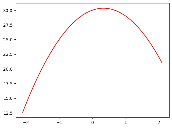

# This simply replicates the same behaviour for each run of this notebook (and your colab if you're following along)
from numpy.random import normal, seed, uniform
np.random.seed(42)

def noise(x,scale): return normal(scale=scale, size=x.shape)
def add_noise(x, mult, add): return x * (1+noise(x,mult)) + noise(x, add)

x = np.linspace(-2,2, num=30)[:,None]
y = add_noise(f(x), 0.1, 1.2)
plt.scatter(x,y)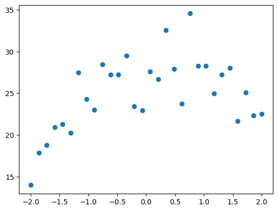

These should look familiar from both Jeremy’s notebook & the previous lessons where we create some quadratics and add noise, lets now show some over and underfitting of these data points.

As Jeremy mentions, we’re going to create a function that fits polynomials of a given degree, a line being degree 1, a quadratic is degree 2, a cubic is degree 3, and so on. He recommends watching this video as a refresher if this jargon is foreign to you. I don’t remember the degrees of a polynomial so I’m going to watch this video now before I continue.

Ok, nice little watch, how long I retain this we’ll see but I’m feeling good about polynomials being chains of terms with co-efficients and variables, thanks mathantics!

from sklearn.linear_model import LinearRegression
from sklearn.preprocessing import PolynomialFeatures
from sklearn.pipeline import make_pipeline

def plot_poly(degree):
    model = make_pipeline(PolynomialFeatures(degree), LinearRegression())
    model.fit(x,y)
    plt.scatter(x,y)
    plot_function(model.predict)
    

plot_poly(1)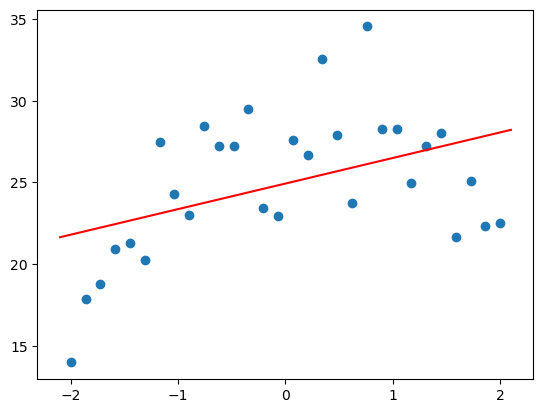

Ok so looks like an “under” fit situation here, we’re not really understanding the relationship between the data points and I don’t think we understand how this data is shaped. Lets look at 10 degrees.

plot_poly(10)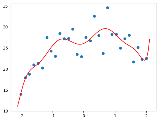

Ok now we’re “over” fitting as we’re simply memorising and far too sensitive to the noise in the data, especially at the end where we completely invert the direction of the line and go back up, this is totally wrong!

Lets now get the right amount of degrees, which is 2 and also plot the underlying true function

plot_poly(2)
plot_function(f, color="b")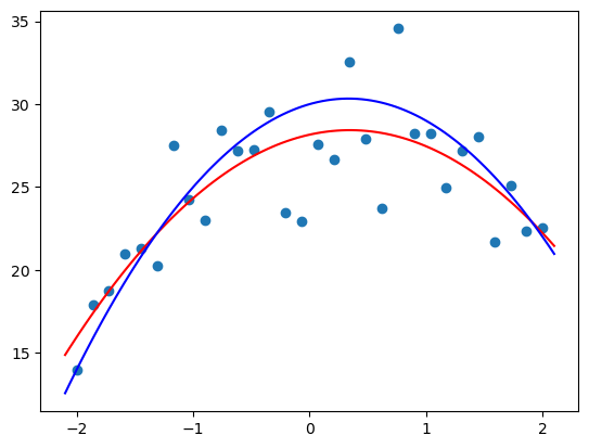

Hey thats pretty cool, we’re not far off here, we’re properly understanding the relationship and estimating correctly the shape of the ‘true’ function. Of course we’re off slightly since there’s noise in the data but the approximation is excitingly close.

Recognising Over/Under Fitting

This takes us back to our validation set, which is the tool we use to figure out if we’re getting this relationship between under and over fitting in the sweet spot. This is a hold out of data from training that we use to see our model might generalise on ‘unseen’ data, we don’t want to use the test set as thats only used at the very end of the process to check on ‘unseen’ unseen data. The problem arises from running many iterations and tests on your validation set, you’re probably going to come across good random variables/parameters as well as slowly leak to your training process, what data is in the validation set which defeats the purpose of trying to see how well your model generalises on data it doesn’t know from training. So we want to make decisions on a good validation set and hold out our test set for the very end of the process.

Transformers uses a “DatasetDict” for holding the training and validation sets. In this scenario we can simply slice apart a random 25% of our dataset for validation, but once again I’ll post Rachel Thomas’s awesome writeup on exactly this question of how to make a good validation set.

dds = tokeniser_dataset.train_test_split(0.25, seed=42)
dds

DatasetDict({
    train: Dataset({
        features: ['id', 'anchor', 'target', 'context', 'labels', 'input', 'input_ids', 'token_type_ids', 'attention_mask'],
        num_rows: 27354
    })
    test: Dataset({
        features: ['id', 'anchor', 'target', 'context', 'labels', 'input', 'input_ids', 'token_type_ids', 'attention_mask'],
        num_rows: 9119
    })
})

Transformers uses the language of our ‘validation’ set being called ‘test’ set which actually isn’t all that uncommon but we’re being specific here so don’t get confused between the two. Remember validation for informing our training process (but not used in the training process to learn from) and the final test set being an ‘unseen’ unseen set to holdout.

Lets modify our test dataset to include the same ‘input’ column that we made for our train dataset

evaluation_df["input"] = 'TEXT1: ' + evaluation_df.context + '; TEXT2: ' + evaluation_df.target + '; ANC1: ' + evaluation_df.anchor
evaluation_ds = Dataset.from_pandas(evaluation_df).map(tokenise_function,batched=True)

Metrics & Correlation

As we worked through in our previous lessons, metrics and loss functions are measurements that we’re able to optimise and very efficiently so. Rachel Thomas has another awesome post about the problems with this efficiency, its definitely worth a read.

An important metric to understand is correlation, how closely or inversely to particular pairs of features rise or fall from each other when the one is changed, there are a couple of cool methods from sklearn that we can use to check out this metric; we can also plot it nicely. Lets bring down the California Housing dataset that comes with sklearn and work with that for starters.

from sklearn.datasets import fetch_california_housing

housing = fetch_california_housing(as_frame=True)
housing = housing["data"].join(housing["target"]).sample(1000, random_state=42)
housing.head()

	MedInc	HouseAge	AveRooms	AveBedrms	Population	AveOccup	Latitude	Longitude	MedHouseVal
20046	1.6812	25.0	4.192201	1.022284	1392.0	3.877437	36.06	-119.01	0.47700
3024	2.5313	30.0	5.039384	1.193493	1565.0	2.679795	35.14	-119.46	0.45800
15663	3.4801	52.0	3.977155	1.185877	1310.0	1.360332	37.80	-122.44	5.00001
20484	5.7376	17.0	6.163636	1.020202	1705.0	3.444444	34.28	-118.72	2.18600
9814	3.7250	34.0	5.492991	1.028037	1063.0	2.483645	36.62	-121.93	2.78000

Ok so we can see some general data about housing in California, lets checkout the correlations with numpy.

np.set_printoptions(precision=2, suppress=True)
np.corrcoef(housing,rowvar=False)

array([[ 1.  , -0.1 ,  0.51, -0.07, -0.  , -0.02, -0.1 ,  0.  ,  0.69],
       [-0.1 ,  1.  , -0.18, -0.11, -0.33,  0.03,  0.03, -0.13,  0.1 ],
       [ 0.51, -0.18,  1.  ,  0.67, -0.06, -0.01,  0.13, -0.05,  0.26],
       [-0.07, -0.11,  0.67,  1.  , -0.04, -0.08,  0.1 , -0.  , -0.04],
       [-0.  , -0.33, -0.06, -0.04,  1.  ,  0.15, -0.11,  0.11, -0.03],
       [-0.02,  0.03, -0.01, -0.08,  0.15,  1.  , -0.17,  0.19, -0.26],
       [-0.1 ,  0.03,  0.13,  0.1 , -0.11, -0.17,  1.  , -0.92, -0.14],
       [ 0.  , -0.13, -0.05, -0.  ,  0.11,  0.19, -0.92,  1.  , -0.06],
       [ 0.69,  0.1 ,  0.26, -0.04, -0.03, -0.26, -0.14, -0.06,  1.  ]])

Here are another few quick ways to get the same matrix and visualise it, natively with pandas, with matplotlib, and seaborn. You can customise these but I think these are nice starts to access the same data

housing.corr()

	MedInc	HouseAge	AveRooms	AveBedrms	Population	AveOccup	Latitude	Longitude	MedHouseVal
MedInc	1.000000	-0.099337	0.509533	-0.068371	-0.003260	-0.021351	-0.099966	0.002959	0.688787
HouseAge	-0.099337	1.000000	-0.184928	-0.108935	-0.333983	0.026371	0.032930	-0.126596	0.099851
AveRooms	0.509533	-0.184928	1.000000	0.666193	-0.055821	-0.009879	0.127917	-0.050235	0.263954
AveBedrms	-0.068371	-0.108935	0.666193	1.000000	-0.041664	-0.082372	0.102355	-0.000441	-0.037114
Population	-0.003260	-0.333983	-0.055821	-0.041664	1.000000	0.152235	-0.110230	0.105513	-0.032120
AveOccup	-0.021351	0.026371	-0.009879	-0.082372	0.152235	1.000000	-0.171743	0.193559	-0.258307
Latitude	-0.099966	0.032930	0.127917	0.102355	-0.110230	-0.171743	1.000000	-0.919229	-0.136581
Longitude	0.002959	-0.126596	-0.050235	-0.000441	0.105513	0.193559	-0.919229	1.000000	-0.063320
MedHouseVal	0.688787	0.099851	0.263954	-0.037114	-0.032120	-0.258307	-0.136581	-0.063320	1.000000

plt.matshow(housing.corr())
plt.show()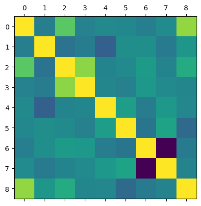

import seaborn as sns

corr = housing.corr()
sns.heatmap(corr)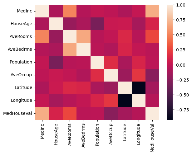

Awesome, we can see that most of the features are fairly uncorrelated but there are some that are highly correlated, for example MedHouseVal and MedInc which are the value of the house and income respectively, lets look into this value specifically

np.corrcoef(housing.MedInc, housing.MedHouseVal)

array([[1.  , 0.69],
       [0.69, 1.  ]])

0.69 is a fairly positive value, lets write a small function to give us back the pair values that we seek.

def correlation(x,y): return np.corrcoef(x,y)[0][1]

correlation(housing.MedInc, housing.MedHouseVal)

0.6887874432146511

Now we can write a small function to plot these pairs and their correlation. Just before we do that, lets look at all the features plotted against each other with seaborns pairplot which can help you at a glance spot some of these nicely matched relationships

sns.pairplot(housing)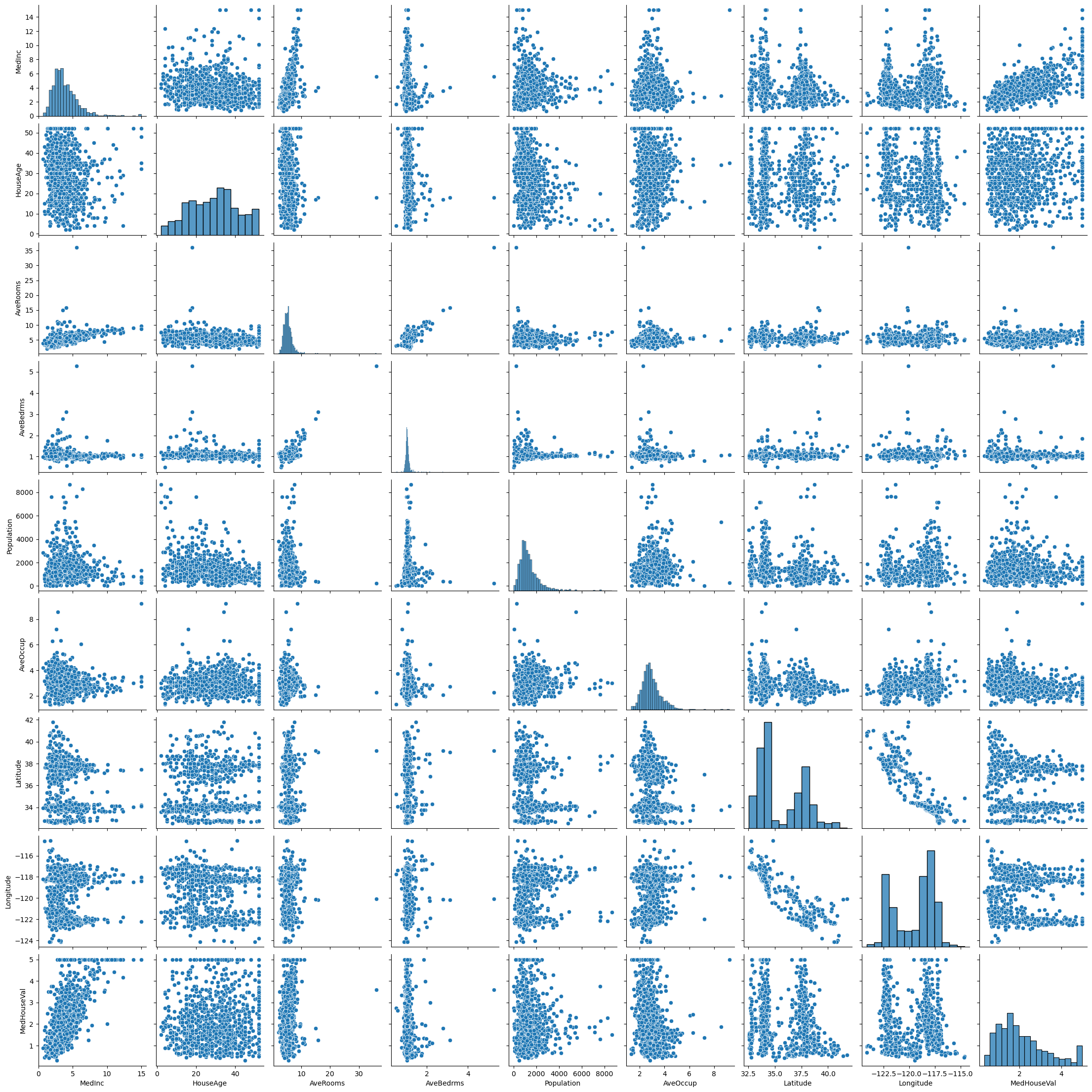

How cool is that, we get a whole bunch of histograms along the diagonal and can see all the other relationships plotted around, however if we want to dig into just one of them, we want to plot it specifically which we’ll make a helper method to do for us.

def show_correlation(df, a, b):
    x,y = df[a], df[b]
    plt.scatter(x,y, alpha=0.5, s=4)
    plt.xlabel(a)
    plt.ylabel(b)
    plt.title(f"{a} vs {b}; Correlation r: {correlation(x,y):.2f}")
    plt.show()
    
show_correlation(housing, "MedInc", "MedHouseVal")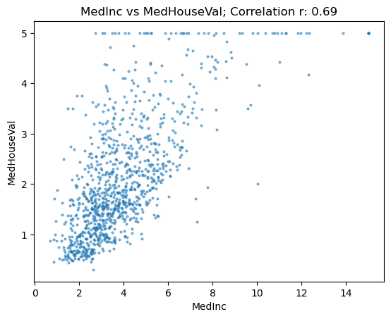

We can see that a bunch of MedHouseVal’s have been clipped at 5 and whilst this is a higher correlation value, there’s still quite a wide spread in the data, lets look at more

show_correlation(housing, "MedInc", "AveRooms")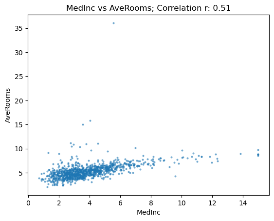

Ok this looks way tighter and more closely matched but we’ve got literally only a value or two as extreme outliers which I suspect are misclassed somehow as Jeremy mentions. Maybe this is a sharehouse or apartment building instead of considering them as different households. Lets filter out the outliers and see what happens to our correlation value.

subset = housing[housing.AveRooms<13]
show_correlation(subset, "MedInc", "AveRooms")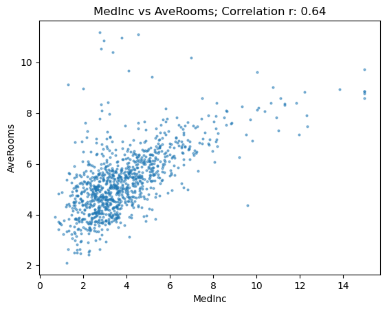

Our value shoots up to 64 and looks highly correlated and tightly plotted rather than spread out. Lets look at another.

show_correlation(subset, "MedHouseVal", "AveRooms")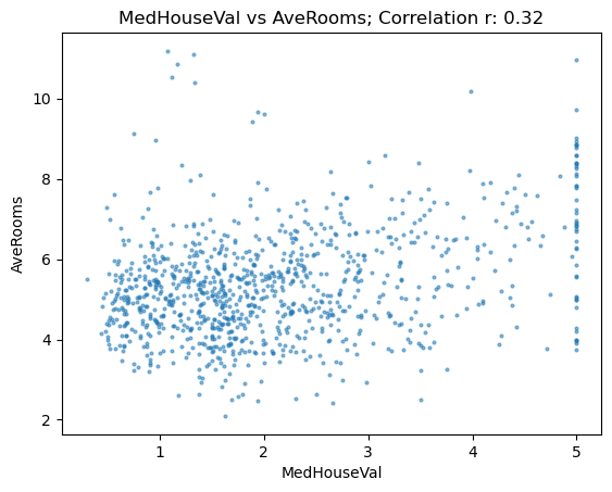

This looks pretty messy and has a pretty weak correlation if any, there’s also that MedHouseVal clipping again.

Lets get back to our Transformers

Transformer Metrics

Transformers expect metrics to be returned as a dictionary, lets create a function to meet this requirement. In our competition we’re using the ‘Pearson Correlation Coefficient’

def correlation_d(eval_pred): return {'pearson':correlation(*eval_pred)}

Training the Transformer

Similar to our fastai learner object we need to create a “Trainer” of which we set the batch size, epochs, learning rate, and other parameters as we would like to manage the training process.

Seems like there’s lots of crossover in terms of techniques and principles, but with some synonyms and similar words used in the same place, ie ‘learner’ is to ‘trainer’.

from transformers import TrainingArguments, Trainer

batch_size = 20
epochs = 2
learning_rate = 8e-5

args = TrainingArguments("outputs",
                        learning_rate=learning_rate,
                        warmup_ratio=0.1,
                        lr_scheduler_type="cosine",
                        fp16=True,
                        evaluation_strategy="epoch",
                        per_device_train_batch_size=batch_size,
                        per_device_eval_batch_size=batch_size*2,
                        num_train_epochs=epochs,
                        weight_decay=0.01,
                        report_to="none")

model = AutoModelForSequenceClassification.from_pretrained(model_name, num_labels=1)
trainer = Trainer(model,
                  args, train_dataset=dds["train"],
                  eval_dataset=dds["test"],
                 tokenizer=tokeniser, compute_metrics=correlation_d)

Some weights of the model checkpoint at microsoft/deberta-v3-xsmall were not used when initializing DebertaV2ForSequenceClassification: ['deberta.embeddings.word_embeddings._weight', 'mask_predictions.classifier.weight', 'lm_predictions.lm_head.LayerNorm.bias', 'mask_predictions.dense.bias', 'mask_predictions.dense.weight', 'lm_predictions.lm_head.dense.bias', 'mask_predictions.LayerNorm.weight', 'lm_predictions.lm_head.bias', 'lm_predictions.lm_head.dense.weight', 'lm_predictions.lm_head.LayerNorm.weight', 'mask_predictions.LayerNorm.bias', 'mask_predictions.classifier.bias']
- This IS expected if you are initializing DebertaV2ForSequenceClassification from the checkpoint of a model trained on another task or with another architecture (e.g. initializing a BertForSequenceClassification model from a BertForPreTraining model).
- This IS NOT expected if you are initializing DebertaV2ForSequenceClassification from the checkpoint of a model that you expect to be exactly identical (initializing a BertForSequenceClassification model from a BertForSequenceClassification model).
Some weights of DebertaV2ForSequenceClassification were not initialized from the model checkpoint at microsoft/deberta-v3-xsmall and are newly initialized: ['pooler.dense.bias', 'classifier.weight', 'classifier.bias', 'pooler.dense.weight']
You should probably TRAIN this model on a down-stream task to be able to use it for predictions and inference.
Using cuda_amp half precision backend

trainer.train()

The following columns in the training set don't have a corresponding argument in `DebertaV2ForSequenceClassification.forward` and have been ignored: target, id, context, input, anchor. If target, id, context, input, anchor are not expected by `DebertaV2ForSequenceClassification.forward`,  you can safely ignore this message.
C:\Users\Nick\Anaconda3\envs\fastai\lib\site-packages\transformers\optimization.py:306: FutureWarning: This implementation of AdamW is deprecated and will be removed in a future version. Use the PyTorch implementation torch.optim.AdamW instead, or set `no_deprecation_warning=True` to disable this warning
  warnings.warn(
***** Running training *****
  Num examples = 27354
  Num Epochs = 2
  Instantaneous batch size per device = 20
  Total train batch size (w. parallel, distributed & accumulation) = 20
  Gradient Accumulation steps = 1
  Total optimization steps = 2736
  Number of trainable parameters = 70830337
You're using a DebertaV2TokenizerFast tokenizer. Please note that with a fast tokenizer, using the `__call__` method is faster than using a method to encode the text followed by a call to the `pad` method to get a padded encoding.

[2736/2736 12:45, Epoch 2/2]

Epoch	Training Loss	Validation Loss	Pearson
1	0.033400	0.030246	0.776644
2	0.021300	0.025342	0.801732

Saving model checkpoint to outputs\checkpoint-500
Configuration saved in outputs\checkpoint-500\config.json
Model weights saved in outputs\checkpoint-500\pytorch_model.bin
tokenizer config file saved in outputs\checkpoint-500\tokenizer_config.json
Special tokens file saved in outputs\checkpoint-500\special_tokens_map.json
Saving model checkpoint to outputs\checkpoint-1000
Configuration saved in outputs\checkpoint-1000\config.json
Model weights saved in outputs\checkpoint-1000\pytorch_model.bin
tokenizer config file saved in outputs\checkpoint-1000\tokenizer_config.json
Special tokens file saved in outputs\checkpoint-1000\special_tokens_map.json
The following columns in the evaluation set don't have a corresponding argument in `DebertaV2ForSequenceClassification.forward` and have been ignored: target, id, context, input, anchor. If target, id, context, input, anchor are not expected by `DebertaV2ForSequenceClassification.forward`,  you can safely ignore this message.
***** Running Evaluation *****
  Num examples = 9119
  Batch size = 40
Saving model checkpoint to outputs\checkpoint-1500
Configuration saved in outputs\checkpoint-1500\config.json
Model weights saved in outputs\checkpoint-1500\pytorch_model.bin
tokenizer config file saved in outputs\checkpoint-1500\tokenizer_config.json
Special tokens file saved in outputs\checkpoint-1500\special_tokens_map.json
Saving model checkpoint to outputs\checkpoint-2000
Configuration saved in outputs\checkpoint-2000\config.json
Model weights saved in outputs\checkpoint-2000\pytorch_model.bin
tokenizer config file saved in outputs\checkpoint-2000\tokenizer_config.json
Special tokens file saved in outputs\checkpoint-2000\special_tokens_map.json
Saving model checkpoint to outputs\checkpoint-2500
Configuration saved in outputs\checkpoint-2500\config.json
Model weights saved in outputs\checkpoint-2500\pytorch_model.bin
tokenizer config file saved in outputs\checkpoint-2500\tokenizer_config.json
Special tokens file saved in outputs\checkpoint-2500\special_tokens_map.json
The following columns in the evaluation set don't have a corresponding argument in `DebertaV2ForSequenceClassification.forward` and have been ignored: target, id, context, input, anchor. If target, id, context, input, anchor are not expected by `DebertaV2ForSequenceClassification.forward`,  you can safely ignore this message.
***** Running Evaluation *****
  Num examples = 9119
  Batch size = 40


Training completed. Do not forget to share your model on huggingface.co/models =)

TrainOutput(global_step=2736, training_loss=0.03071680386164035, metrics={'train_runtime': 767.9404, 'train_samples_per_second': 71.24, 'train_steps_per_second': 3.563, 'total_flos': 160758836273364.0, 'train_loss': 0.03071680386164035, 'epoch': 2.0})

Holy Batman there’s a lot more logging going on for transformers, but I’m sure this would be useful as soon as you’ve got to debug or solve some problems, regardless our loss is going down and our coefficient is going up. Lets make some predictions of which we could submit if we wanted to compete

preds = trainer.predict(evaluation_ds).predictions.astype(float)
preds[:5]

The following columns in the test set don't have a corresponding argument in `DebertaV2ForSequenceClassification.forward` and have been ignored: target, id, context, input, anchor. If target, id, context, input, anchor are not expected by `DebertaV2ForSequenceClassification.forward`,  you can safely ignore this message.
***** Running Prediction *****
  Num examples = 36
  Batch size = 40

array([[0.5 ],
       [0.7 ],
       [0.22],
       [0.29],
       [0.05]])

preds.max(), preds.min()

(1.09765625, -0.007724761962890625)

We’ve got predictions above 1 and below 0 which are impossible so lets clip them. I think in the future, we’re better off using sigmoid which Jeremy seems to allude to but thats for another day.

preds = np.clip(preds, 0, 1)

preds.max(), preds.min()

(1.0, 0.0)

Awesome, nicely limited.

OK we made it through the notebook, this was really familiar as Jeremy noted and didn’t feel too new. The experience of finding a great model to transfer learn, kickoff the training loop and look at the loss metrics is a comfortable space to be. Other than needing to take in tokenisation and numericalisation, this all felt pretty friendly. Its fascinating how the same concepts, behaviours, mindset, and generally the code can be re-used to predict shark species from images or classify documents from text. Its kind of mind blowing!

I was maybe expecting more of a discussion on the structure of transformers and why they’re unique compared to other architectures like ULMFit which Jeremy mentioned but maybe thats for a later lesson, its also something that I’m obviously free to research myself. Maybe another blog to write once I’m further through the course and come back to, nonetheless lets crack out the textbook.

Book Content

Self-Supervised Learning

Self Supervision is the process of learning from data without explicit labels, in the example from fastbook, its noted that the chapter introduction model has read a bunch of prior words from a document and attempts to predict the next word. This process doesn’t have explicit labels but the model is learning these ‘labels’ from the actual training data itself. We’ve worked through a normal supervised task above via transfer learning and some labelled data and this is explicitly different from self-supervision. Here is an example of self-supervision for a vision task that Jeremy notes in the book, I’m going to reference this post to describe some of the self supervision topics we come across. From this blog, the self supervision description is ‘train a model using labels that are naturally part of the input data, rather than requiring separate external labels.’ As usual I couldn’t say it better.

Ok so our goal is to run this self-supervised training process to discover some ‘innate’ weights that are useful, we then transfer learn to our new task and fine tune on the original intended goal. ULMFit once again turns up as a great example of this process, I think it would be fun to re-create this paper down the track, might be a fun series to do in general.

Pre-Text and Down-Stream Tasks

The ‘pre-training’ task that discovers these innate weights I was paraphrasing before is called the ‘pretext’ task, the fine tuning tasks intended for our original goal are called ‘downstream’ tasks. Some of the vision pretext tasks mentioned in the computer vision example are colorisation, placing subsets of an image in the correct location, placing frames in the right order, in-painting where you fill in a missing portion of an image, and classifying corrupted images. Have a look at the linked post above for visual examples of these tasks.

Naturally deciding on these pretext tasks is important and Jeremy discusses how you want to decide some process where ‘if solved’ it would provide some insight into the original task you’re trying to complete.

Consistency Loss

Jeremy discusses a topic called “consistency loss” or “noise contrastive estimation” in computer vision. In a lot of these pretext tasks, you have some original input, you then muck with it, make it greyscale for example in the colorisation task, and then ask the model to predict the colors and compare it to the original input. For these tasks you want the original input and the ‘pre-texted’ image to match as you’re just trying to re-construct the original input, you’d also hope that the same original input that is augmented in different batches for different amounts still produces the same output since the augmentations are from the same input and are only different in terms of the randomness applied to the colorisation or patching or rotation etc. Apparently you can add to the loss function an penalising term that punishes ‘getting different answers for different versions of the same data.’ From Jeremy’s post he says they used 1000x less labeled data and smashed the previous state of the art, apparently you can add this to any pretext task and since its so effective, why wouldn’t you?!

There’s lots of awesome papers in this post, as I mentioned before when I was thinking of re-creating ULMFit sometime, I think doing a write up on self-supervision and this consistency loss would be fun and interesting.

Tokenisation With Fastai

Ok we’ve understood tokenisation and numericalisation from working through the huggingface notebook so I won’t rehash these topics here but the book provides a great guide on how to use the fastai library and build some tokenisers so I’m keen to see how its different from huggingface, lets get stuck in.

from fastai.text.all import *

path = untar_data(URLs.IMDB)

files = get_text_files(path, folders = ["train", "test", "unsup"])

txt = files[42].open().read(); txt[:500]

"I wanted to like this movie. I really, really did. I was so excited when I saw the preview, which scared the hell out of me. But when I saw the actual film, I was disappointed. The acting is stilted, and the attempts at comedy are woefully out of place and forced. And I'm sorry, but a boy being chased by a turd in a bedpan is not funny or scary, it's just stupid. I grew up on the Bell Witch legend, so I know quite a bit about it. A lot of facts in the movie are right on target, but this film sho"

Ok this review is hilarious, “a boy being chased by a turd” is apparently a real scene in this movie and dissapointingly the reviewer said it wasn’t funny or scary, what a shame, so much potential.

As of when the book was written, spaCY is the english word tokeniser used which is apparently driven by a sophisticated rules engine containing special rules for URLs, special english words etc. Rather than calling spaCY directly with the ‘SpacyTokenizer’, we’re going to use the fastai ‘WordTokenizer’ which will point to fastai’s current default tokeniser. I wonder if there’s an obvious way to inspect this object and see what fastai is currently using as of now (15th Jan 23) when I’m writing this.

tokeniser = WordTokenizer()
tokens = first(tokeniser([txt]))
print(coll_repr(tokens, 30))

(#224) ['I','wanted','to','like','this','movie','.','I','really',',','really','did','.','I','was','so','excited','when','I','saw','the','preview',',','which','scared','the','hell','out','of','me'...]

As we saw in the previous tokenisation task from the lecture, we mainly get all the words split out with some special cases handled, uppercase, and fullstops modified. As noted in the book, there are so many subtle rules of langauge that are implicit and explicit in how we write, its extremely fluid and complex but there are underlying principles in the structure that we want noted and specified, like names needing uppercase, or a word at the start of the sentence vs in the middle of a sentence having different meanings.

doc(coll_repr)

coll_repr

coll_repr(c, max_n=10)

String repr of up to `max_n` items of (possibly lazy) collection `c`

Show in docs

coll_repr is a cool way to show a python collection as well as its size instead of wrapping all the boilerplate calls to structure it, it also uses the fastcore ‘L’ class which is python lists on steroids, super useful stuff!

tokeniser

<fastai.text.core.SpacyTokenizer at 0x1f83cf16fb0>

Looks like SpacyTokenizer is still king of the throne, I wonder if and when this will be changed and for what reason!

fastai_tokeniser = Tokenizer(tokeniser)
print(coll_repr(fastai_tokeniser(txt), 30))

(#239) ['xxbos','i','wanted','to','like','this','movie','.','i','really',',','really','did','.','i','was','so','excited','when','i','saw','the','preview',',','which','scared','the','hell','out','of'...]

Ok there’s some extra functionality being wrapped ontop here, as noted in the book, in particular the ‘xxbos’ token which means the start of a new text, ‘BOS’ in the broader NLP space is an acronym that means “beginning of stream.” Supposedly this helps the model realise that it needs to forget what it was thinking about and focus on the upcoming words as this is a new document/text. This tokenisation process definitely seems to standardise and structure any text into an explicit version where a lot of implicit rules of written language are explicitly expressed as tokens. An example being the start of a sentence which we as people have no need to signify other than a capital letter and a full stop prior but are extremely valuable tokens for a model to explicitly pickup.

Some other tokens of significance are ‘xxmaj’ meaning the next word starts uppercase and by default all the text is set to lowercase, ‘xxunk’ meaning the next word is unknown. We can also checkout the rules that are used and I assume that this list can be modified or added to if need be. We can always inspect these rules with the doc() function or ?? jupyter magic calls as we’ve done throughout the previous couple of chapters.

defaults.text_proc_rules

[<function fastai.text.core.fix_html(x)>,
 <function fastai.text.core.replace_rep(t)>,
 <function fastai.text.core.replace_wrep(t)>,
 <function fastai.text.core.spec_add_spaces(t)>,
 <function fastai.text.core.rm_useless_spaces(t)>,
 <function fastai.text.core.replace_all_caps(t)>,
 <function fastai.text.core.replace_maj(t)>,
 <function fastai.text.core.lowercase(t, add_bos=True, add_eos=False)>]

doc(replace_rep)

replace_rep

replace_rep(t)

Replace repetitions at the character level: cccc -- TK_REP 4 c

Show in docs

replace_rep??

Signature: replace_rep(t)
Source:   
def replace_rep(t):
    "Replace repetitions at the character level: cccc -- TK_REP 4 c"
    def _replace_rep(m):
        c,cc = m.groups()
        return f' {TK_REP} {len(cc)+1} {c} '
    return _re_rep.sub(_replace_rep, t)
File:      c:\users\nick\anaconda3\envs\fastai\lib\site-packages\fastai\text\core.py
Type:      function

Subword Tokenisation

For a language like english where most, if not all words are separated by a space, this method of tokenisation where we splitup mostly by word is quite effective, however in languages like Mandarin, Hungarian, Turkish, Japanese, etc that don’t have the same rules in terms of spaces or joining multiple words together, different techniques are required. One of those is subword tokenisation which is done by the following steps:

Analyse a corpus of documents and find the most commonly occurring groups of letters, this is your vocab
Tokenise the corpus using this vocab of subword units

This honestly did not occur to me as significant in terms of language differences regarding structure and moreso seemed important for compound words in the english language or words derived from latin where multiple latin roots are joined together. An example being animal taxonomy like we worked through in the lecture. Either way lets work through a quick example with Jeremy and the book.

txts = L(o.open().read() for o in files[:500])

Lets instantiate our tokeniser, with a custom vocab size which we can set, we then need to ‘train’ it by reading our documents and finding the common sequences to make the vocab. We use fastai’s setup() function that is apparently called automatically during data processing pipelines but we’re going to manually call here.

def subword(size):
    sp = SubwordTokenizer(vocab_sz=size)
    sp.setup(txts)
    return " ".join(first(sp([txt]))[:40])

subword(1000)

'▁I ▁want ed ▁to ▁like ▁this ▁movie . ▁I ▁really , ▁really ▁did . ▁I ▁was ▁so ▁ex c it ed ▁when ▁I ▁saw ▁the ▁pre vi e w , ▁which ▁sc ar ed ▁the ▁he ll ▁out ▁of ▁me'

If we have a smaller vocab, each token will represent fewer characters and more tokens will be needed to represent a sentence

subword(200)

'▁I ▁w an t ed ▁to ▁like ▁this ▁movie . ▁I ▁re al ly , ▁re al ly ▁ d i d . ▁I ▁was ▁s o ▁ e x c it ed ▁w he n ▁I ▁s a w'

Vice versa for larger and the most common english words will turn up in the vocab itself, hence needing less to represent a sentence.

%%time

subword(10_000)

CPU times: total: 656 ms
Wall time: 428 ms

'▁I ▁want ed ▁to ▁like ▁this ▁movie . ▁I ▁really , ▁really ▁did . ▁I ▁was ▁so ▁excited ▁when ▁I ▁saw ▁the ▁preview , ▁which ▁scare d ▁the ▁hell ▁out ▁of ▁me . ▁But ▁when ▁I ▁saw ▁the ▁actual ▁film'

Ok my intuition was completely the opposite, I felt like if you had a smaller vocab, you’d need the tokens to represent ‘more’ of the sentence but I’m wrong, in order to represent the sentence, if you’ve only got ~200 special tokens that have to represent everything, you’ll end up just making pairs/singles of letters since thats the maximum you can encode. This is an interesting problem for building a good vocab, there must be some sweet spot as I assume you’d want to represent the language in the smallest way possible for efficiency but maybe not, food for thought for now. The book discusses how this allows you to scale between character tokenisation that I’ve just mentioned (small subword vocab) and word tokenisation (large vocab), whilst also being language agnostic since you can just subword any length of text.

Interestingly Jeremy raises that this tokenisation approach can be used to handle other ‘languages’ like genomic sequences or MIDI music notation, I guess these are ‘structured’ languages representing genes and music respectively. Fascinating!

Numericalisation with Fastai

This is the process of mapping all our tokens to numbers which can be fed into our neural nets, we can simply set the numerical value of each token to the index of the vocab. I do wonder if you’d want to sort this vocab in some way, like putting punctuation together or words that are similar together in space but maybe this provides no utility. I think this would be done with an embedding matrix but we’ve seemingly jumped ahead to chapter 10 in the book and I remember from the other year that this was done together through the lectures but we haven’t come across embeddings in the course yet. I have no doubt it will be discussed however.

We need to call setup() again on Numericalise in order to create the vocab and give numbered values to our tokens

tokens = fastai_tokeniser(txt)
print(coll_repr(fastai_tokeniser(txt),31))

(#239) ['xxbos','i','wanted','to','like','this','movie','.','i','really',',','really','did','.','i','was','so','excited','when','i','saw','the','preview',',','which','scared','the','hell','out','of','me'...]

tokens200 = txts[:200].map(fastai_tokeniser)
tokens200[0]

(#207) ['xxbos','xxmaj','once','again','xxmaj','mr','.','xxmaj','costner','has'...]

Numericalize?

Init signature:
Numericalize(
    self,
    vocab=None,
    min_freq=3,
    max_vocab=60000,
    special_toks=None,
)
Docstring:      Reversible transform of tokenized texts to numericalized ids
File:           c:\users\nick\anaconda3\envs\fastai\lib\site-packages\fastai\text\data.py
Type:           _TfmMeta
Subclasses:

num = Numericalize()
num.setup(tokens200)
coll_repr(num.vocab,20)

"(#1968) ['xxunk','xxpad','xxbos','xxeos','xxfld','xxrep','xxwrep','xxup','xxmaj','the','.',',','a','and','of','to','is','it','i','in'...]"

nums = num(tokens)[:20]; nums

TensorText([   2,   18,  613,   15,   43,   20,   25,   10,   18,   79,   11,
              79,   87,   10,   18,   27,   56, 1269,   76,   18])

TensorText?

Init signature: TensorText(x, **kwargs)
Docstring:      Semantic type for a tensor representing text
File:           c:\users\nick\anaconda3\envs\fastai\lib\site-packages\fastai\text\data.py
Type:           _TensorMeta
Subclasses:     LMTensorText

How cool, there’s a tensor class specifically for handling text within fastai, awesome. We can also see the magical numbers representing our tokens, this gives us our ability to transform between numbers and text.

Batching Text Data

A significant set of choices and challenges arise in the image work we did in previous chapters because we have to feed our neural net with tensors of the same shape, meaning we had to resize, pad, crop, chop, and modify our images to suit the architecture we chose. How do we achieve the same in text documents when we can’t just ‘resize’ a sentence, and the order of our text is really important since they’re connected in a chain together within a sentence. We need one batch to start where the last finished.

The way this is handled is by following this series of steps: 1. Randomise the order of inputs (movie reviews) so at the beginning of an epoch, we have shuffled entries, creating a new stream for each epoch 2. Transform the individual texts (a single movie review) into a stream by concatenating them together (one super review containing all reviews in a random order). Note that each review itself is not shuffled but the order of the reviews within the entire stream. 3. Cut this stream into a certain number of batches (our batch size chooses this). A working example being, if a stream has 50,000 tokens and we set a batch size of 10, we will have 10 mini streams of 5,000 tokens. The token order will be preserved so the first mini-stream is 0-5000 tokens, second mini-stream is 5001-10_000 etc. Remember ‘xxbos’ token is added at the start of each stream so the model knows when we have a new text.

The most important take-away from this process is that there’s an ‘inner-state’ that the model will remember between batches so that it will produce the same activations no matter the sequence length we pick. This is me paraphrasing the book and in even simpler language it looks like we just chop up the whole text into small blocks and just remember that we’re still working on a ‘stream’ between batches instead of an entirely new text document.

Fastai sorts all this out for us with the LMDataLoader, lets work through that now

nums200 = tokens200.map(num)
dl = LMDataLoader(nums200)

x,y = first(dl)
x.shape, y.shape

(torch.Size([64, 72]), torch.Size([64, 72]))

Sizes look good, now our y should just be our x data offset by one word since our task is to predict only the next word in a piece of text.

" ".join(num.vocab[o] for o in x[0][:20])

'xxbos xxmaj once again xxmaj mr . xxmaj costner has dragged out a movie for far longer than necessary .'

" ".join(num.vocab[o] for o in y[0][:21])

'xxmaj once again xxmaj mr . xxmaj costner has dragged out a movie for far longer than necessary . xxmaj aside'

Cool, our next token is xmaj but I’ve grabbed one more index so that we can see we get one more word with the offset.

Language Model DataBlocks

Lets use the TextBlock DataBlock to do a lot of the heavy lifting for us, remember that we’ve got to get our pre-trained wikipedia model and fine-tune it to the corpus of language relative to what we’re trying to predict which is imdb reviews before actually fine tuning the model to our task.

get_imdb = partial(get_text_files, folders=["train", "text", "unsup"])

dls_lm = DataBlock(blocks=TextBlock.from_folder(path, is_lm=True),
                  get_items=get_imdb,
                  splitter=RandomSplitter(0.1)).dataloaders(path,
                                                           path=path,
                                                           bs=128,
                                                           sequential_len=80)

Lets checkout a batch as we would whenever making a dataloader before going through our training loop.

dls_lm.show_batch(max_n=2)

	text	text_
0	xxbos me , my boyfriend , and our friend watched this " movie " if that s what u wanna call it , and we agree with the last person , but we were stupid and bought the damn thing , we thought it really was about diablo so we bought it . \n\n we hate it xxmaj really xxup xxunk xxrep 31 ! so beware : xxup do xxup not xxup	me , my boyfriend , and our friend watched this " movie " if that s what u wanna call it , and we agree with the last person , but we were stupid and bought the damn thing , we thought it really was about diablo so we bought it . \n\n we hate it xxmaj really xxup xxunk xxrep 31 ! so beware : xxup do xxup not xxup buy
1	, sure this wo n't appeal everyone comedy has changed the past decade if a comedy does n't have any controversial meaning or non stop sex , fart jokes then its not funny but to everyone who can take a joke its a must buy or at least a rental . \n\n i recommended this movie to my friends and family and they all enjoyed it , maybe we 're from another	sure this wo n't appeal everyone comedy has changed the past decade if a comedy does n't have any controversial meaning or non stop sex , fart jokes then its not funny but to everyone who can take a joke its a must buy or at least a rental . \n\n i recommended this movie to my friends and family and they all enjoyed it , maybe we 're from another planet

Fine-Tuning the Language Model

And we’re back on familiar ground where we build a learner object, pass an architecture, set some metrics etc and kick off our training loop

learn = language_model_learner(dls=dls_lm,
                               arch=AWD_LSTM,
                               drop_mult=0.3,
                               metrics=[accuracy, Perplexity()]).to_fp16()

100.00% [105070592/105067061 00:01<00:00]

By default the language learner uses cross-entropy loss which we haven’t studied within the course yet but I bet has been mentioned earlier in the book if you read it linearly. You can think of what we’re doing as a classification problem if you think of our vocab as the possible categories, the ‘Perplexity()’ metric that we’ve added is often used in NLP and its simply the exponential of the cross entropy loss ‘torch.exp(cross_entropy)’.

Since this cross-entropy metrics isn’t very intuitive to understand past ‘bigger is badder and smaller is gooder’, Jeremy includes the accuracy function so we have some intuition of how many words we predict are actually correct. He also makes the statement that the cross-entropy loss ‘tells us more about the model’s confidence than its accuracy’ which is a really interesting statement I hope to have better intuition on in the future.

As usual we want to run the fit_one_cycle() method which includes all kinds of smarts in terms of scheduling the learning rates and freezing/unfreezing the pre-trained weights.

learn.fit_one_cycle(5, 2e-3)

epoch	train_loss	valid_loss	accuracy	perplexity	time
0	4.123974	4.040399	0.291216	56.848999	21:02
1	4.011928	3.937155	0.298377	51.272511	21:09
2	3.953815	3.903160	0.300778	49.558800	21:12
3	3.920171	3.889413	0.302054	48.882202	21:17
4	3.903158	3.887264	0.302198	48.777275	21:27

Another interesting bit of jargon is the ‘encoder’ which the book explains as ‘the model not including the final layer’ and of which the learner object has an API for, being save_encoder(). Intuitively this means you get to keep the model but without the task specific final layer at the head of the model, meaning you have the useful ‘body’ of the model and you can simply add a new head to the model and fine tune for a new task whenever you want.

Generating Reviews

Our model is actually capable of creating a review with a prompt to start and a specified length with some randomness so that we get different reviews.

text = "I liked this movie because"
n_words = 40
n_sentences = 2
preds = [learn.predict(text, n_words, temperature=0.75) for _ in range(n_sentences)]

print("\n".join(preds))

i liked this movie because it was so good . If you have a good idea , you might buy it . It should have been based on a true story and this movie will not be the same as the previous remake
i liked this movie because it 's a great movie . i saw it several times , and i guess it is great . This is good enough for me . It is a shame when i saw it but it was very

text = "I'm a big boy"

preds = [learn.predict(text, n_words, temperature=0.75) for _ in range(n_sentences)]

print("\n".join(preds))

I 'm a big boy , but i just ca n't believe enough to be married to Gary Cooper , Gary Cooper , Walter Pidgeon ( in a film that 's n't Cooper 's ) . i would
I 'm a big boy , but i have heard of a lot of movies from the 30 's and a lot of stuff . In a lot of movies , i was more of a child than i was . At the

text = "Edward Norton sometimes can"

preds = [learn.predict(text, n_words, temperature=0.75) for _ in range(n_sentences)]

print("\n".join(preds))

Edward Norton sometimes can be peaked as an actor . In this case , he had to play it with a variety of occasionally unlikely ambitions . He was a star in Anthony Hopkins ' play , which was made
Edward Norton sometimes can not describe a new English name , but it seems that he is really English . He says , " i am writing this review " . The English writers of " the White

text = "the simpsons are"

preds = [learn.predict(text, n_words, temperature=0.75) for _ in range(n_sentences)]

print("\n".join(preds))

the simpsons are always funny when they are in trouble . They are the best of all and enjoy the movie . The humour is limited to those who might enjoy for the audience . Like documentaries , they do
the simpsons are a bit much different from the usual American and American sitcoms , but there are many other gags that are so funny , especially at the Deadtime Stories series . One of the funniest ,

text = "Terminator is my"

preds = [learn.predict(text, n_words, temperature=0.75) for _ in range(5)]

print("\n".join(preds))

Terminator is my favorite Terminator film , but it is hardly a good thing . The story makes nothing much sense and is not about the buoyancy of a nuclear plant . The Terminator is not a bit of
Terminator is my favorite Terminator film , and one of the worst sci - fi films ever . The movie was made with a very low budget , low budget , and expensive special effects and artificial digital effects .
Terminator is my favorite of all time . 

 It 's a great choice for this movie to watch ! i think it has more interesting questions than the rest of the film , but i do n't understand why they were
Terminator is my favorite of all the Terminator movies , and it 's an excellent story ; it 's the only one that will make you laugh , he 's got someone from the Icarus 3 to attack . This
Terminator is my favorite Terminator film and it is one of the best action films ever made . I 'm not sure why it 's a sequel or a remake . It was n't a good movie but i guess

text = "Alien scared me because"

preds = [learn.predict(text, n_words, temperature=0.75) for _ in range(5)]

print("\n".join(preds))

Alien scared me because he was so dumb , it did n't break in the way this plane was advanced . i thought we had to be able to fill up the space space , but i was n't afraid to cut the filming
Alien scared me because they were all mind - numbing . This movie could have been much better if you did n't expect the movie to be incredibly boring and not bad . It 's not the only thing that 's just
Alien scared me because there was no way for anyone to annoy me . In the first half of the movie it was the one who kept the kids . The only one that Roger Ebert has to say is
Alien scared me because of the fact that the Alien aliens / aliens and aliens are the only reason for fighting a Alien earth , and this one really just made it feel like it was being made … that 's actually
Alien scared me because it made me laugh . This movie is so bad that there 's a look for it . Watching this movie , i thought it sounded like a documentary about a man who was kidnapped by aliens with

These are kind of stunningly good, yes there are some quirks and issues with the sentences but its a lot of original feeling content and posts. I wonder if we can tune further and see if the text prompts get better anecdotally.

learn.fit_one_cycle(5, 2e-3)

epoch	train_loss	valid_loss	accuracy	perplexity	time
0	3.910050	3.890951	0.301302	48.957420	21:16
1	3.930783	3.879690	0.302058	48.409214	21:12
2	3.872207	3.868199	0.303140	47.856113	21:28
3	3.849681	3.861700	0.303823	47.546116	21:25
4	3.839549	3.860545	0.303930	47.491245	21:29

text = "Yeah Mr.White, Yeah Science"

preds = [learn.predict(text, n_words, temperature=0.75) for _ in range(5)]

print("\n".join(preds))

Yeah xxunk , Yeah Science Fiction Shows Gone Too Much ! THE REAL NAME OF THE WHO OF THE
Yeah xxunk , Yeah Science . Oh yeah , the Bugs Bunny version of Star Wars , which is a great horror flick , is about a Russian scientist who is teenage and wants to be a Russian
Yeah xxunk , Yeah Science Fiction . This is the least - made TV film that I 've ever seen . Well , it 's one of the most enjoyable science fiction films i 've seen . 

 And
Yeah xxunk , Yeah Science Fiction . 

 Worst of all : I 'm sure i did n't want to explain this movie . 

 i mean , i thought it was a good idea to watch this film … i have
Yeah xxunk , Yeah Science Fiction is based on the character of Othello , and is very interesting as i believe it is based on the true Shakespeare . Just like Shakespeare 's Hamlet , Shakespeare 's "

I’ve made the mistake of starting with an unknown token which isn’t split nicely “Mr.White” when I should have instead run something like “Mr White”.

Anyway this isn’t exactly what we came for but its super cool! Lets move on to the classifier instead.

Creating the Classifier DataLoaders

Our language model at this point predicts the next word of a document and doesn’t need any labels, as this self-supervised work inherently gives you what you’re looking for. However we want to classify the sentiment of a document instead, lets make our DataBlock for just such a task.

dls_clas = DataBlock(blocks=(TextBlock.from_folder(path, vocab=dls_lm.vocab), CategoryBlock),
                     get_y = parent_label,
                     get_items=partial(get_text_files, folders = ["train", "test"]),
                     splitter=GrandparentSplitter(valid_name="test")).dataloaders(path, path=path, bs=16, seq_len=72)

dls_clas.show_batch(max_n=3)

	text	category
0	xxbos xxmaj match 1 : xxmaj tag xxmaj team xxmaj table xxmaj match xxmaj bubba xxmaj ray and xxmaj spike xxmaj dudley vs xxmaj eddie xxmaj guerrero and xxmaj chris xxmaj benoit xxmaj bubba xxmaj ray and xxmaj spike xxmaj dudley started things off with a xxmaj tag xxmaj team xxmaj table xxmaj match against xxmaj eddie xxmaj guerrero and xxmaj chris xxmaj benoit . xxmaj according to the rules of the match , both opponents have to go through tables in order to get the win . xxmaj benoit and xxmaj guerrero heated up early on by taking turns hammering first xxmaj spike and then xxmaj bubba xxmaj ray . a xxmaj german xxunk by xxmaj benoit to xxmaj bubba took the wind out of the xxmaj dudley brother . xxmaj spike tried to help his brother , but the referee restrained him while xxmaj benoit and xxmaj guerrero	pos
1	xxbos xxmaj heavy - handed moralism . xxmaj writers using characters as mouthpieces to speak for themselves . xxmaj predictable , plodding plot points ( say that five times fast ) . a child 's imitation of xxmaj britney xxmaj spears . xxmaj this film has all the earmarks of a xxmaj lifetime xxmaj special reject . \n\n i honestly believe that xxmaj jesus xxmaj xxunk and xxmaj julia xxmaj xxunk set out to create a thought - provoking , emotional film on a tough subject , exploring the idea that things are not always black and white , that one who is a criminal by definition is not necessarily a bad human being , and that there can be extenuating circumstances , especially when one puts the well - being of a child first . xxmaj however , their earnestness ends up being channeled into preachy dialogue and trite	neg
2	xxbos xxmaj the movie " macarthur " begins and ends at xxmaj gen . xxmaj douglas macarthur 's , xxmaj gregory xxmaj peck , xxmaj alma xxmaj mata the xxup us xxmaj military xxmaj academy of xxmaj west xxmaj point on the xxmaj hudson . xxmaj we see a frail 82 year old xxunk give the commencement speech to the graduating class of 1962 about what an honor it is to serve their country . xxmaj the film then goes into an almost two hour long flashback on xxmaj gen . macarthur 's brilliant as well as controversial career that starts in the darkest hours of xxup wwii on the besieged island of xxmaj corregidor in the xxmaj philippines in the early spring of 1942 . \n\n xxmaj told to leave he island for xxmaj australia before the xxmaj japanese military invade it xxmaj gen . macarthur for the very	pos

learn = text_classifier_learner(dls_clas,
                               AWD_LSTM,
                               drop_mult=0.5,
                               metrics=accuracy).to_fp16()

Now I’ve neglected to do one important thing:

Save the encoder from my earlier language model training

This prevents me from performing the fast fine-tuning that I would woto_detachthrough with the book. I’ll add in the applied code and write through some explanations of what they’re doing and what kind of output we’d expect but apologies as my baby 2GB GPU can’t handle these large modelling tasks and I’m currently writing late at night and don’t want to re-spin up a colab session to retrain over an hour or so. I may come back to this once I’ve built my planned ‘beast’ training rig and rerun these tasks.

Fine-Tuning the Classifier

Here is where we would run the following:

Load the encoder
Freeze up to the last two layers
Fit one cycle to set the final two layer weights more appropriately
Unfreeze some more layers and continue training
Unfreeze the entire model and continue training

Lets look at what this code would look like from the book

Loading the encoder

learn = learn.load_encoder("finetuned.pk1")

Freeze up to the last two layers

learn.freeze_to(-2)

Fit one cycle to set the two final layer weights more appropriately

learn.fit_one_cycle(1, 2e-2)

Unfreeze some more layers and continue training

Note here the book shows slicing as a way of providing different learning rates for different parts of the model. I’m not quite sure why the book chooses these particular values but I’m sure we’ll dive deeper into why this learning rate discrimination has been chosen. This topic is called “discriminative layer training”, here’s a nice fastai forum post on the topic and the docs themselves explaining the topic as well as this gradual unfreezing technique.

learn.freeze_to(-3)
learn.fit_one_cycle(n_epoch=1,
                    lr_max=slice(1e-2/(2.6**4), 1e-2))

Unfreeze the entire model and continue training

learn.unfreeze()
learn.fit_one_cycle(2, slice(1e-3/(2.6**4),1e-3))

The final subtitle of this chapter discusses the danger of these kind of language models, in particular the impact they had on the FCC repealing net neutrality and how its many online comments were likely generated by these sorts of language models as justification for the law changing. I won’t rehash this discussion here as Jeremy and Rachel do a far better job of describing these ethical considerations than I will but I want to only write a final note as encouragement to checkout the dangers of language models. In particular the current discussion is about GPT3 and how school kids etc are cheating at exams and homework using this tool, its generating a lot of legible but nonsensicle language that looks legitimate on first glance but is often riddled with errors. In particular meta had to take down their scientific paper model ‘Galactica’ because it was basically espousing nonsense whilst seemingly being very convincing. It had learned how to talk the talk in terms of scientific research but was writing absolute junk, there’s good discussions on twitter and well written journalist posts about the problems of these large language models.

In our misinformation and poor media literacy age, these are fascinating but concerning times.